Use Tikhonov Regularization to Solve Fredholm Integral Equation

Background #

Fredholm in­te­gral equa­tion of the first kind is writ­ten as,

$f(x)=\int_{a}^{b}K(x,s)p(s)\mathrm{d}s.$

The prob­lem is to find $p(s)$, given that $f(x)$ and $K(x,s)$ are known. This equa­tion oc­curs quite of­ten in many dif­fer­ent ar­eas.

Discretization-based Method #

Here we de­scribe a dis­cretiza­tion-based method to solve the Fredholm in­te­gral equa­tion. The in­te­gral equa­tion is ap­prox­i­mately re­placed by a Riemann sum­ma­tion over grids,

$f(x_i)=\sum_j \Delta_s K(x_i, s_j) p(s_j)$

where $\Delta_s$ is the grid size along the di­men­sion $s$ and $x_i$, $s_j$ are the grid points with $i$ and $j$ in­di­cat­ing their in­dices. When grid size $\Delta_s\to0$, the sum­ma­tion con­verges to the true in­te­gral. It is more con­ve­nient to write it in the ma­trix form,

$\boldsymbol{f} = \boldsymbol{\Delta}_s \boldsymbol{K} \boldsymbol{p}$

where

$\boldsymbol{f}=(f(x_1), f(x_2),\cdots,f(x_n))^{\mathrm{T}},$

$\boldsymbol{K}= \begin{pmatrix} K(x_1,s_1) & K(x_1,s_2) & \cdots & K(x_1,s_m) \\ K(x_2,s_1) & K(x_2,s_2) & \cdots & K(x_2,s_m) \\ \vdots & \vdots & \ddots & \vdots \\ K(x_n,s_1) & K(x_n,s_2) & \cdots & K(x_n,s_m) \end{pmatrix}$

$\boldsymbol{p} = (p(s_1),p(s_2),\cdots,p(s_m))^{\mathrm{T}}$

and $\boldsymbol{\Delta}_s = \Delta_s \boldsymbol{I}$ with $\boldsymbol{I}$ be­ing the iden­tity ma­trix of di­men­sion $n \times n$.

Now solv­ing the Fredholm in­te­gral equa­tion is equiv­a­lent to solv­ing a sys­tem of lin­ear equa­tions. The stan­dard ap­proach or­di­nary least squares lin­ear re­gres­sion, which is to find the vec­tor $\boldsymbol{p}$ min­i­miz­ing the norm $\vert\vert \boldsymbol{\Delta}_s \boldsymbol{K} \boldsymbol{p}-\boldsymbol{f}\vert\vert_2^2$. In prin­ci­ple, the Fredholm in­te­gral equa­tion may have non-unique so­lu­tions, thus the cor­re­spond­ing lin­ear equa­tions are also ill-posed. The most com­monly used method for ill-posed prob­lem is Tikhonov reg­u­lar­iza­tion which is to min­i­mize

$\vert\vert\boldsymbol{\Delta}_s \boldsymbol{K} \boldsymbol{p}-\boldsymbol{f}\vert\vert_2^2+\alpha^2\vert\vert\boldsymbol{p}\vert\vert_2^2$

Note that this is ac­tu­ally a sub­set of Tikhonov reg­u­lar­iza­tion (also called Ridge reg­u­lar­iza­tion) with $\alpha$ be­ing a pa­ra­me­ter.

When $p(s)$ is a prob­a­bil­ity den­sity func­tion #

In many cases, both $f(x)$ and $g(s)$ are prob­a­bil­ity den­sity func­tion (PDF), and $K(x,s)$ is a con­di­tional PDF, equiv­a­lent to $K(x\vert s)$. Thus, there are two con­straints on the so­lu­tion $p(s)$, that is $p(s)\geq 0$ and $\int p(s)\mathrm{d}s = 1$. These two con­straints trans­late to $p(s_i)\geq 0$ for any $s_i$ and $\Delta_s\sum_i p(s_i)=1$. Hence, we need to solve the Tikhonov reg­u­lar­iza­tion prob­lem sub­ject to these two con­straints.

In the fol­low­ing, I will show how to solve the Tikhonov reg­u­lar­iza­tion prob­lem with both equal­ity and in­equal­ity con­straints. First, I will show that the Tikhonov reg­u­lar­iza­tion prob­lem with non-neg­a­tive con­straint can be eas­ily trans­lated to a reg­u­lar non-neg­a­tive least square prob­lem (NNLS) which can be solved us­ing ac­tive set al­go­rithm.

Let us con­struct the ma­trix,

$\boldsymbol{A}= \begin{pmatrix} \Delta_s \boldsymbol{K} \\ \alpha \boldsymbol{I} \end{pmatrix}$

and the vec­tor,

$\boldsymbol{b}= \begin{pmatrix} \boldsymbol{f}\\ \boldsymbol{0} \end{pmatrix}$

where $\boldsymbol{I}$ is the $m\times m$ iden­tity ma­trix and $\boldsymbol{0}$ is the zero vec­tor of size $m$. It is easy to show that the Tikhonov reg­u­lar­iza­tion prob­lem $\mathrm{min}(\vert\vert\boldsymbol{\Delta}_{s} \boldsymbol{K} \boldsymbol{p} - \boldsymbol{f}\vert\vert_{2}^{2}+\alpha^2\vert\vert\boldsymbol{p}\vert\vert_{2}^{2})$ sub­ject to $\boldsymbol{p}\geq 0$ is equiv­a­lent to the reg­u­lar NNLS prob­lem,

$\mathrm{min}(\vert\vert\boldsymbol{A}\boldsymbol{p}-\boldsymbol{b}\vert\vert_2^2),\mathrm{\ sub­ject\ to\ }\boldsymbol{p}\geq 0$

Now we add the equal­ity con­straint, $\Delta_s\sum_i p(s_i)=1$ or $\boldsymbol{1}\boldsymbol{p}=1/\Delta_s$ writ­ten in ma­trix form. My im­ple­men­ta­tion of solv­ing such prob­lem fol­lows the al­go­rithm de­scribed in Haskell and Hanson ^[1]. According to their method, the prob­lem be­comes an­other NNLS prob­lem,

$\mathrm{min}(\vert\vert\boldsymbol{1}\boldsymbol{p}-1/\Delta_s\vert\vert_2^2+\epsilon^2\vert\vert\boldsymbol{A}\boldsymbol{p}-\boldsymbol{b}\vert\vert_2^2),\mathrm{\ sub­ject\ to\ }\boldsymbol{p}\geq 0$

The so­lu­tion to the above equa­tion con­verges to the true so­lu­tion when $\epsilon\to0^+$. Now I have de­scribed the al­go­rithm to solve the Fredholm equa­tion of the first kind when $p(s)$ is a prob­a­bil­ity den­sity func­tion. I call the al­go­rithm de­scribed above as non-neg­a­tive Tikhonov reg­u­lar­iza­tion with equal­ity con­straint (NNETR).

Code #

Here I show the core code of the al­go­rithm de­scribed above.

# core algorithm of non-negative equality Tikhonov regularization (NNETR)
def NNETR(K, f, Delta, epsilon, alpha):
    # the first step
    A_nn = np.vstack((K, alpha * np.identity(K.shape[1])))
    b_nn = np.hstack((f, np.zeros(K.shape[1])))

    # the second step
    A_nne = np.vstack((epsilon * A_nn, np.full(A_nn.shape[1], 1.0)))
    b_nne = np.hstack((epsilon * b_nn, 1.0))

    # Use NNLS solver provided by scipy
    sol, residue = scipy.optimize.nnls(A_nne, b_nne)

    # solution should be divided by Delta (grid size)
    sol = sol/Delta
    return sol, residue

Examples #

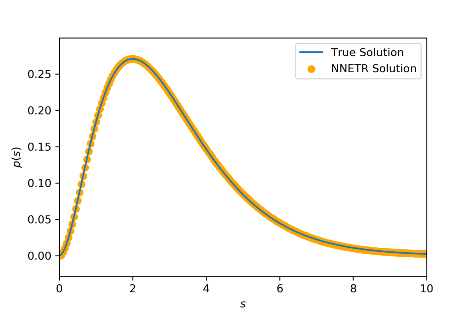
• Compounding an ex­po­nen­tial dis­tri­b­u­tion with its rate pa­ra­me­ter dis­trib­uted ac­cord­ing to a gamma dis­tri­b­u­tion yields a Lomax dis­tri­b­u­tion $f(x)=a(x+1)^{-(a+1)}$, sup­ported on $(0,\infty)$, with $a>0$. $k(x,\theta)=\theta e^{-\theta x}$ is an ex­po­nen­tial den­sity and $p(\theta) = \Gamma(a)^{-1}\theta^{a-1}e^{-\theta}$ is a gamma den­sity.

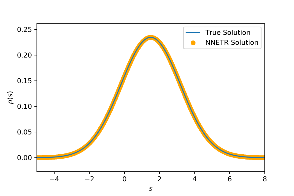
• Compounding a Gaussian dis­tri­b­u­tion with mean dis­trib­uted ac­cord­ing to an­other Gaussian dis­tri­b­u­tion yields (again) a Gaussian dis­tri­b­u­tion $f(x)=\math­cal{N}(a,b^2+\sigma^2)$. $k(x\vert\mu)=\math­cal{N}(\mu,\sigma^2)$ and $p(\mu)=\math­cal{N}(a,b^2)$

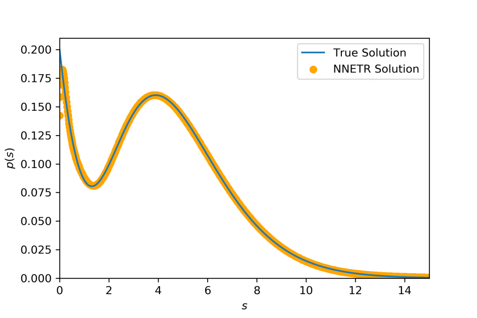
• Compounding an ex­po­nen­tial dis­tri­b­u­tion with its rate pa­ra­me­ter dis­trib­uted ac­cord­ing to a mix­ture dis­tri­b­u­tion of two gamma dis­tri­b­u­tions. Similar to the first ex­am­ple, we use $k(x,\theta)=\theta e^{-\theta x}$. But here we use $p(\theta)=q p(\theta\vert a_1)+(1-q)p(\theta\vert a_2)$ where $q$, $a_1$ and $a_2$ are pa­ra­me­ters. It is clear that $p(\theta)$ is a mix­ture be­tween two dif­fer­ent gamma dis­tri­b­u­tions such as it is a bi­modal dis­tri­b­u­tion. Following the first ex­am­ple, we have $f(x)=qf(x\vert a_1)+(1-q)f(x\vert a_2)$ where $f(x\vert a)=a(x+1)^{-(a+1)}$.

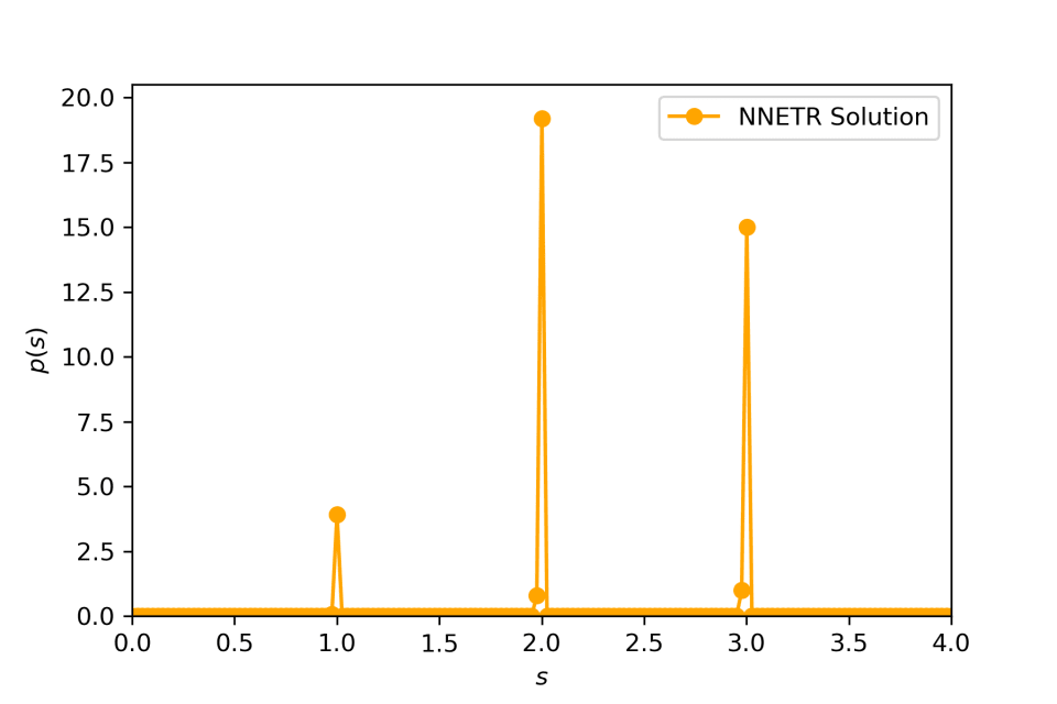
• Compounding an ex­po­nen­tial dis­tri­b­u­tion with its rate pa­ra­me­ter dis­trib­uted as a dis­crete dis­tri­b­u­tion.